The detail about Attention structure
this is the detail about attention structure
Attention Structure
Scaled Dot-Product Attention
The attention architecture derives from the mechanisms of human attention. When an image is placed in front of a human, the human scans the global image to obtain areas that are worth focusing on, and devotes more attention to these areas to obtain information. Nowadays, the popular attention model generally relies on the encoder-decoder framework, which can deal with tasks including NLP, image processing, etc.

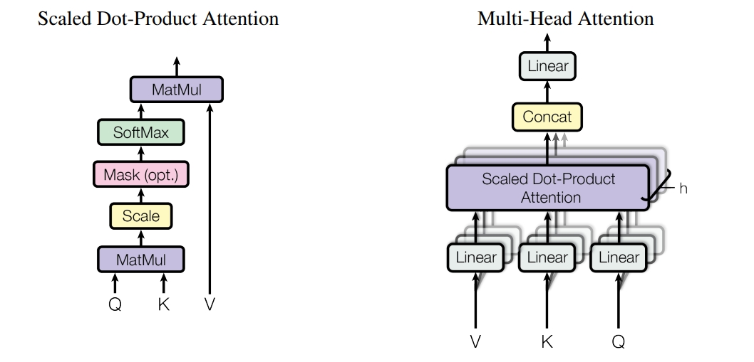
Scaled Dot-Product Attention is the most basic attention structure. Multi-Head Attention is multiple parallel Scaled Dot-Product Attention, which splices the output of each Scaled Dot-Product Attention and does a linear transformation to output.

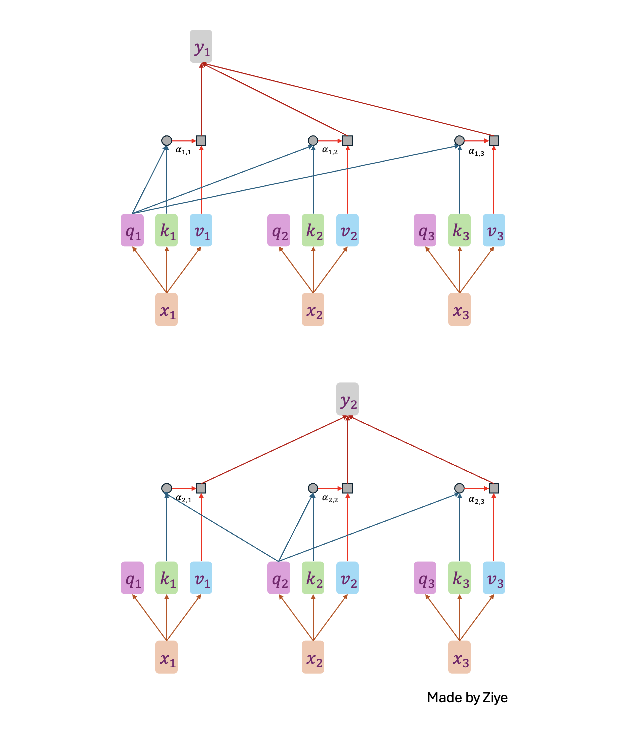
Attention can be considered as a specific word weighting, given a sequence of inputs \(\{x_1, x_2, \dots, x_n\}\), after the attentions layer, combining the input individuals \(\{x_1, x_2, \dots, x_n\}\) and outputs \(\{y_1, y_2, \dots, y_n\}\) will be as follows:
- The input features are multiplied by three sets of weight matrices \(W^Q, W^K, W^V\) to generate the three matrices of query, key, and value;
- The attention weight matrix \(A\) is obtained from the product of a certain \(Q\) and \(K\), which is normalized to get \(\hat{A}\);
- The normalized weights \(\hat{A}\) are multiplied by V to get the final output feature \(O\).

Mathematically, the self-attention matrix for input matrices \((Q, K, V)\) is calculated as:
\[\text{Attention}(Q, K, V) = \text{softmax}\left(\frac{QK^T}{\sqrt{d_k}}\right) V\]
Multi-Head Attention
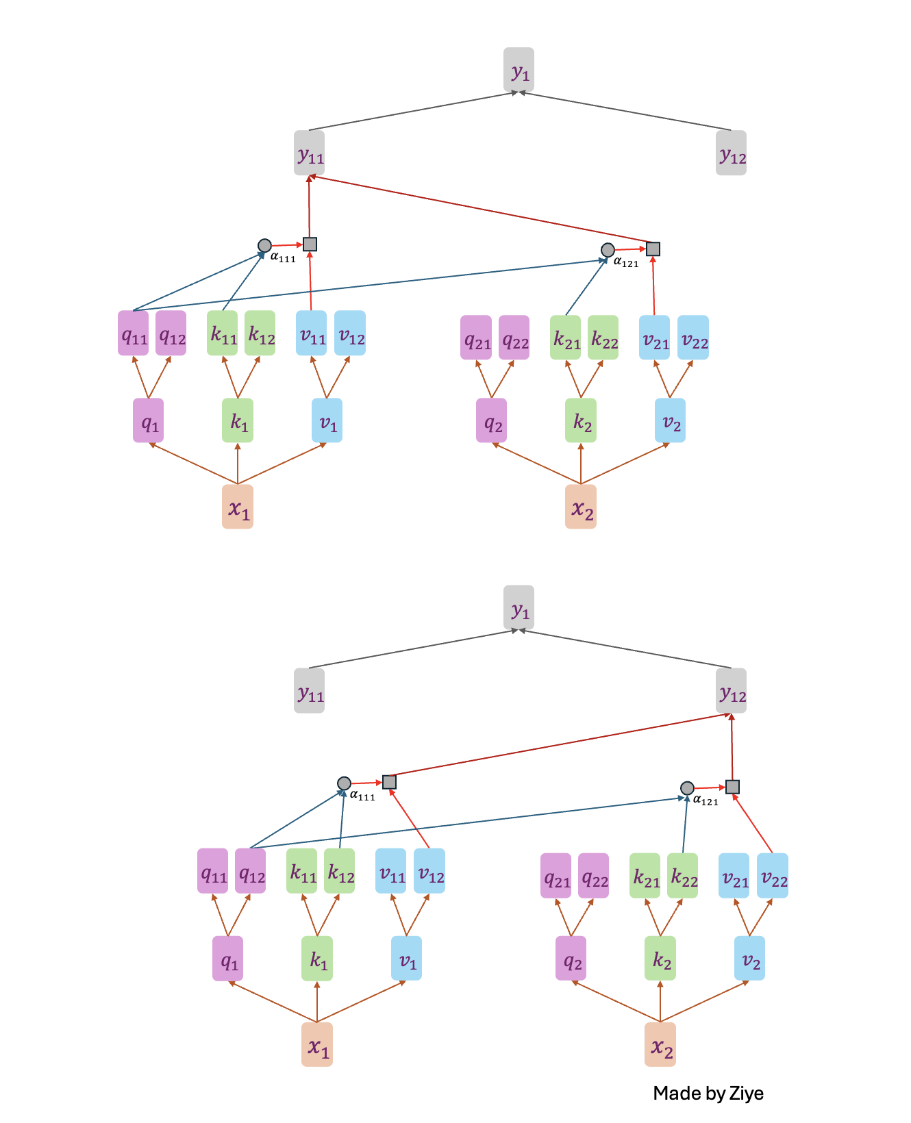
If each vector \(q_i, k_i, v_i\) is split into n, we can get the n-headed attention mechanism. It is recognized that multi-head self-attention mechanisms are better than single-head ones because it can capture information in more dimensions.

At the beginning, we need to import some libraries we will normally use.
import torch
from torch import nn
import torch.functional as F
import math
We need some data for testing. The dimension of testing data is 3.
- The first dimension represents batch.
- The second dimension represents time.
- The third dimension represnts the dimension after Encoder.
And in language model, the ‘512’ below normally means the dimensions of the word vector do you want to map your word to after Embedding.
X = torch.randn(128,64,512) #Batch, Time, Dimension
print(X.shape)
Next, we set up the basic parameters of Multihead attention.
- d_model represents the number of dimensions I want to map to the QKV space.
- n_head repersents the number of head.
d_model = 512
n_head = 8
class multi_head_attention(nn.Module):
# When we are writing a pytorch class, we need to inherit nn.Module
    def __init__(self, d_model, n_head) -> None:
        super(multi_head_attention, self).__init__() # Initialize some basic parameters

        self.d_model = d_model
        self.n_head = n_head

        self.w_q = nn.Linear(d_model, d_model) #Query
        self.w_k = nn.Linear(d_model, d_model) #Key
        self.w_v = nn.Linear(d_model, d_model) #Value
        # It's like we are looking for some queries to match some keys, and values are then weighted to combine.

        self.w_combine = nn.Linear(d_model, d_model)
        # Because of 'multi-head', we need a combinatorial mapping of the outputs.

        self.softmax = nn.Softmax(dim=-1)
#Still in class multi_head_attention(nn.Module):
    def forward(self, q, k, v, mask = None):
        batch, time, dimension = q.shape # get the dimensions of Q, K, V
        n_d = self.d_model // self.n_head # Because we have n heads, 'd_model' for each submodel has to be divisible by 'n_head'.
        q, k, v = self.w_q(q), self.w_k(k), self.w_v(v)

        q = q.view(batch, time, self.n_head, n_d).permute(0, 2, 1, 3)
        k = k.view(batch, time, self.n_head, n_d).permute(0, 2, 1, 3)
        v = v.view(batch, time, self.n_head, n_d).permute(0, 2, 1, 3)
        # We cannot put 'n_head' in the last dimension because we need to process the last two dimensions.

        score = q @ k.transpose(2, 3) / math.sqrt(n_d) # The most important code in Attention.

        minusInfty = -10000
        if mask is not None:
            score = score.masked_fill(mask == 0, minusInfty)
        score = self.softmax(score) @ v

        score = score.permute(0, 2, 1, 3).contiguous().view(batch, time, dimension)

        output = self.w_combine(score)

        return output
attention = multi_head_attention(d_model, n_head)
output = attention(X, X, X)
print(output, output.shape)
Something you might want to know about Attention
The square root of d in the Attention calculation
Why should we divide \(\sqrt{d}\) in the Attention calculation?
Assume that the Query vector \(q\) and the Key vector \(k\) have dimension \(d\) and their elements are independent and identically distributed random variables with mean \(0\) and variance \(1\).
Then their dot product \(q \cdot k\) can be expressed as: \(q \cdot k = \sum_{i=1}^d q_i k_i\). Since each \(q_i\) and \(k_i\) is an independently and identically distributed random variable, their product \(q_i k_i\) is also a random variable. For each \(q_i k_i\), the expectation is \(0\) and the variance is \(1\).
Therefore, the expected value of the dot product \(q \cdot k\) is:
\[\mathbb{E}[q \cdot k] = \mathbb{E} \left[ \sum_{i=1}^d q_i k_i \right] = \sum_{i=1}^d \mathbb{E}[q_i k_i] = 0\]Moreover, its variance is:
\[\text{Var}(q \cdot k) = \text{Var} \left( \sum_{i=1}^d q_i k_i \right) = \sum_{i=1}^d \text{Var}(q_i k_i) = d\]Thus, the standard deviation of the dot product \(q \cdot k\) is:
\[\sigma = \sqrt{\text{Var}(q \cdot k)} = \sqrt{d}\]By the Central Limit Theorem, the sum of these independently and identically distributed random variables will converge to a normal distribution when $d$ is large enough. To normalize this, we subtract the expected value and divide by the standard deviation:
\[\frac{q \cdot k - \mathbb{E}[q \cdot k]}{\sqrt{\text{Var}(q \cdot k)}}\]Here, \(\mathbb{E}[q \cdot k] = 0\) and \(\text{Var}(q \cdot k) = d\), so the expression becomes:
\[\frac{q \cdot k}{\sqrt{d}}\]This will make the expression approximately obey the standard normal distribution \(N(0, 1)\).