Introduction to KAN

this is an introduction about KAN

KAN and MLP

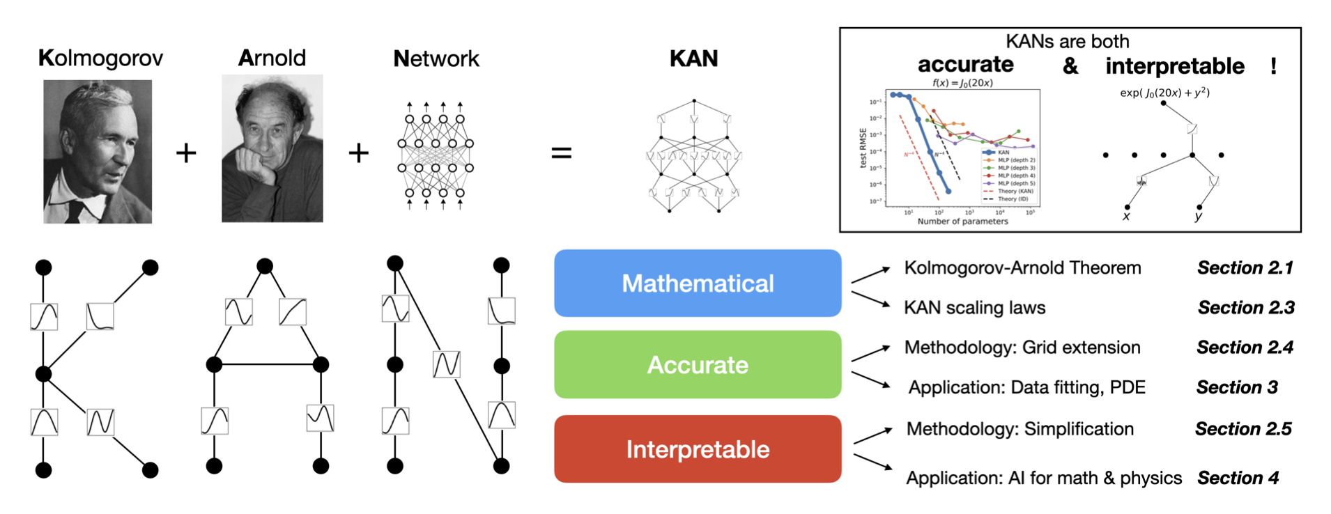
The emergence of the KANs (Kolmogorov-Arnold Networks) model has led to heated discussions in the AI community, and the reason for this is that the flaws in the structure of the MLPs itself have been troubling the researchers involved.

Nowadays, most AI research is based on MLP. The appearance of KANs can potentially revolutionize the direction of AI research. If KANs are as marvelous as expected in subsequent research, their appearance will be like the emergence of cement in a society that has been only using wood to build houses.

The drawbacks of MLP

The theoretical basis for MLPs is that a single hidden layer network containing enough neurons can approximate any continuous function. But MLPs have some natural flaws:

Vanishing and exploding gradients

Vanishing gradients: the gradient tends to zero, the network weights cannot be updated or are updated very slightly, and the network will not be effective even if it is trained for a long time;

Exploding gradient: the gradient grows exponentially and becomes very large, leading to a large update of the network weights, making the network unstable.

Whether the gradient disappears or the gradient explosion is essentially due to the backpropagation of the deep neural network.

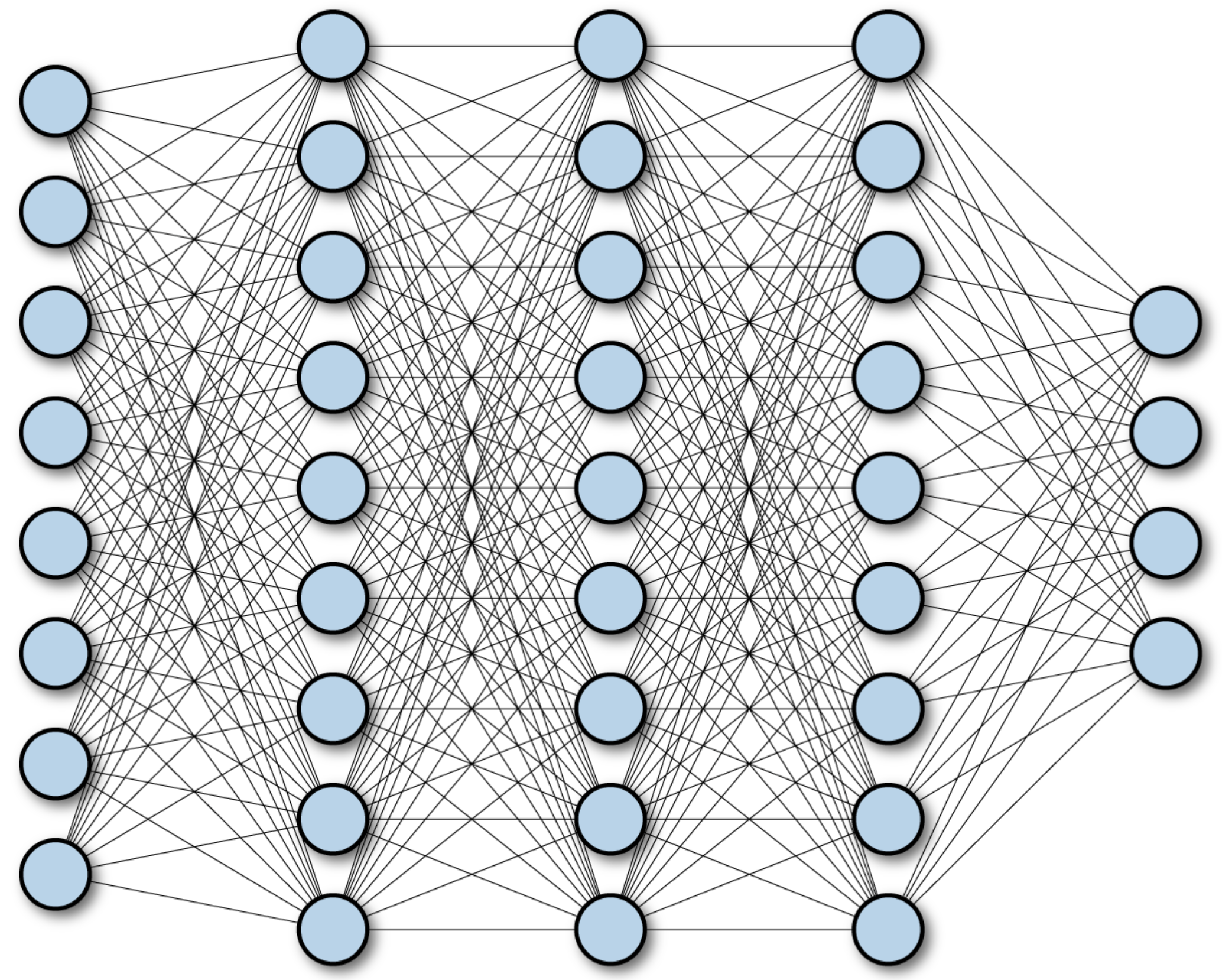
For example, in a four-layer neural network, its backpropagation formula is as follows:

\[\frac{\partial L}{\partial w_1} = \frac{\partial L}{\partial y_4} \frac{\partial y_4}{\partial z_4} \frac{\partial z_4}{\partial y_3} \frac{\partial y_3}{\partial z_3} \frac{\partial z_3}{\partial y_2} \frac{\partial y_2}{\partial z_2} \frac{\partial z_2}{\partial y_1} \frac{\partial y_1}{\partial z_1} \frac{\partial z_1}{\partial w_1}\] \[\frac{\partial L}{\partial y_4} = \sigma'(z_4) w_4 \sigma'(z_3) w_3 \sigma'(z_2) w_2 \sigma'(z_1) x_1\]

where \(y_i = \sigma(z_i) = \sigma(w_i x_i + b_i)\), which \(x_i = y_{i-1}\), and \(\sigma\) is sigmoid activation function.

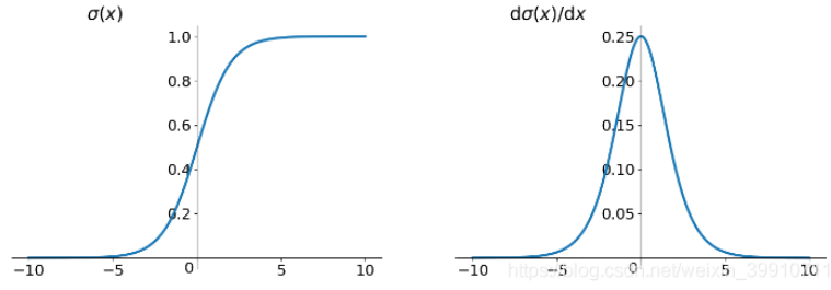
From the above, it can be seen that there is a sequence of multiplications in the backpropagation of the neural network. Also, the derivative of the sigmoid activation function has a value range of 0 to 0.25. So when each \(w_i\) is small, and there are many \(\sigma'\) multiplied together, the gradient tends to 0. When each \(w_i\) very large, the gradient becomes very large.

While many methods say they solve this problem, the issue is still complicated to avoid completely, as it is an intrinsic shortcoming of MLPs.

Inefficient utilization of parameters

MLPs usually use fully connected networks, so the number of parameters is huge. When the network becomes very deep, only a few parameters are utilized. And this is one reason why LLM may have reached a dead end.

Although it is possible to simplify the structure using CNNs or regularization or the like, essentially, the structure of a highly dense continuous linear model coupled with an activation function dictates that the MLP can’t be too sparse or will not have enough representational power.

Inadequate capacity to handle high-dimensional data and Long-term dependency issues

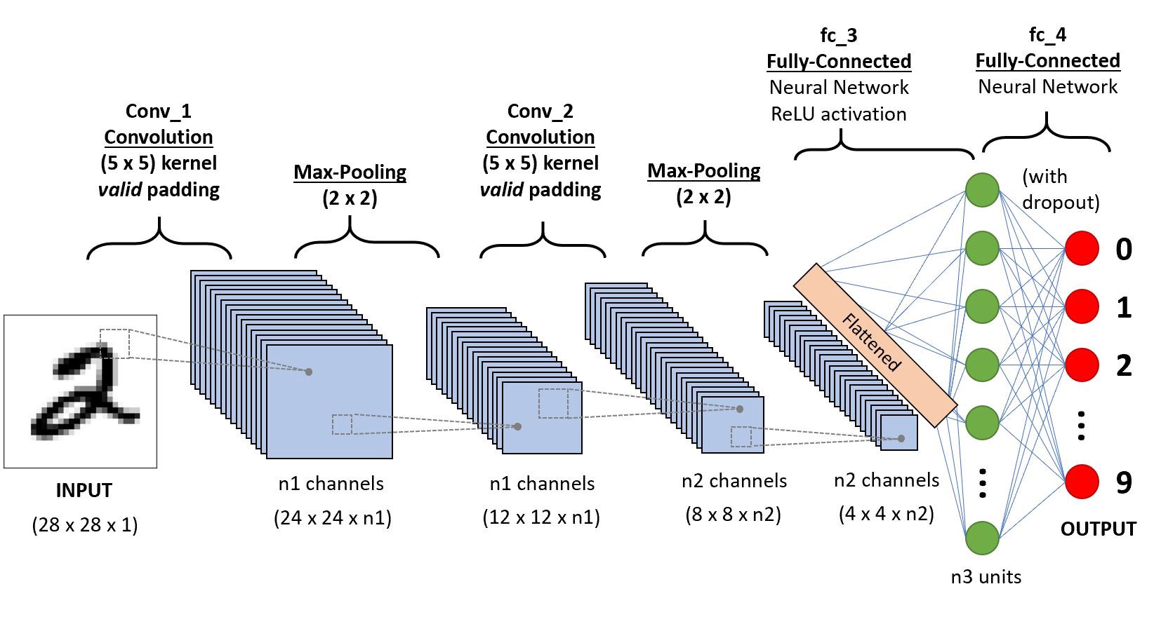
MLPs do not utilize the intrinsic structure of the data, such as local spatial correlations in images and sequence information in textual data. Although CNN and RNN can improve these problems, this base module of MLPs determines that these problems cannot be solved completely.

MLPs also have difficulty capturing long-standing relationships in input sequences. (RNN & Transformer can improve it)

Kolmogorov-Arnold Networks

The Kolmogorov-Arnold representation theorem

KANs are inspired by the Kolmogorov-Arnold representation theorem. Vladimir Arnold and Andrey Kolmogorov established that if f is a multivariate continuous function on a bounded domain, then f can be written as a finite composition of continuous functions of a single variable and the binary operation of addition.

More specifically, for a smooth \(f : [0, 1]^n \rightarrow \mathbb{R}\),

\[f(\mathbf{x}) = f(x_1, \dots, x_n) = \sum_{q=1}^{2n+1} \Phi_q \left( \sum_{p=1}^n \phi_{q,p}(x_p) \right)\]

where \(\phi_{q,p} : [0,1] \rightarrow \mathbb{R}\) and \(\Phi_q : \mathbb{R} \rightarrow \mathbb{R}\). This theorem reveals how any multivariate continuous function can be represented by a simpler set of functions.

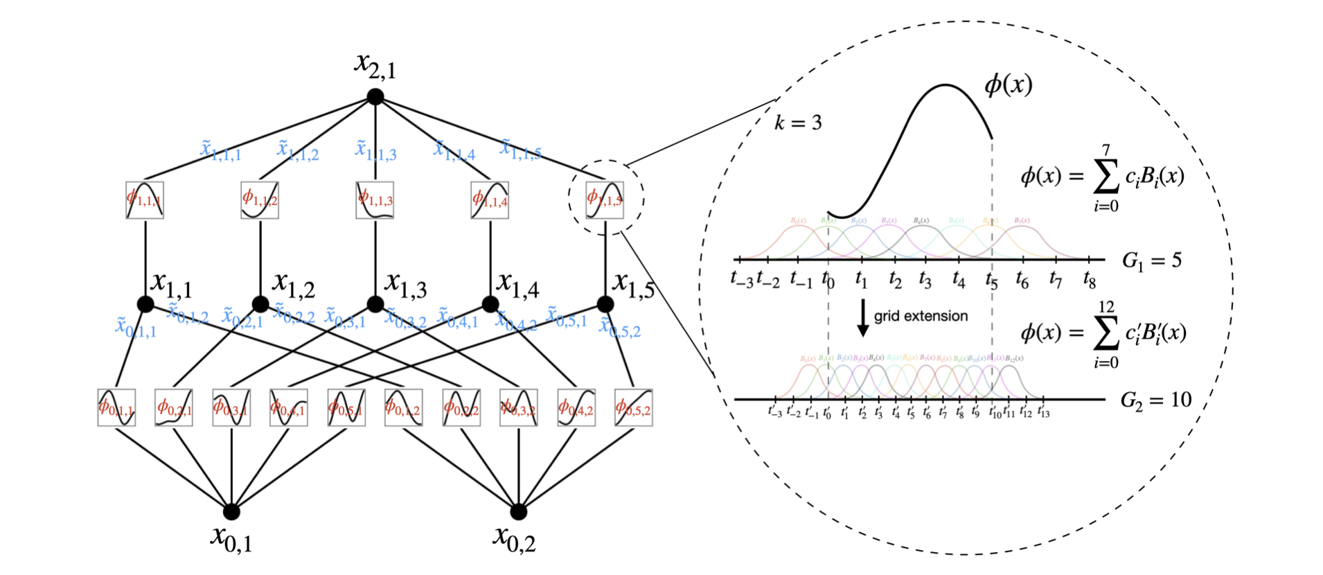
It can be shown that the Kolmogorov-Arnold representation theorem is a simple KANs which has only two-layer nonlinearities and a small number of terms (2n + 1) in the hidden layer. This structure appeared a long time ago, but the difficulty is how to make the KANs deeper. And two-layer networks are too simple to approximate complex functions. (Details of deepening KANs will be mentioned later)

Why KANs are awesome

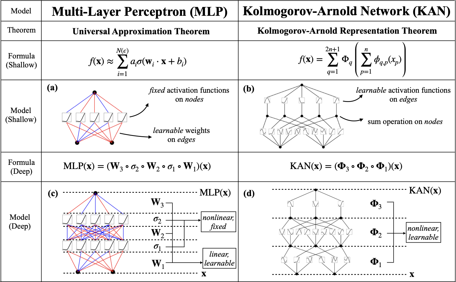
KANs contrast MLPs by not having a nested relationship between activation functions and parameter matrices but rather a nesting of directly nonlinear functions \(\Phi\). And \(\Phi\) all use the same function structure. (In the paper, they use the spline function in numerical analysis)

\[KAN(x) = (\Phi_{L-1} \circ \Phi_{L-2} \circ \cdots \circ \Phi_1 \circ \Phi_0)x\] \[MLP(x) = (W_{L-1} \circ \sigma \circ W_{L-2} \circ \sigma \circ \cdots \circ W_1 \circ \sigma \circ W_0)x\]

When learning the network parameters, MLPs learn the linear function with a fixed nonlinear activation function. In contrast, KANs learn the parameterized nonlinear function directly, which enhances their characterization ability.

Because of the parameters’ complexity, although individual spline functions are more complex to learn than linear functions, KANs typically allow for smaller computational graphs than MLPs (i.e., a smaller network size is required to achieve the same effect).

The details about KANs

If MLPs fit a function with some lines, KANs fit a function with some curves. In KANs, the spline function is used as the nonlinear function \(\Phi\).

The KAN layer is simply a matrix of functions \(\Phi = \{ \phi_{q,p} \}\), \(p=1,2,\cdots,n_{\text{in}}\), $$q=1,2,\cdots,n_{\text{out}}.

\[\Phi_l = \left( \begin{array}{ccc} \phi_{l,1,1}(\cdot) & \phi_{l,1,2}(\cdot) & \cdots & \phi_{l,1,n_l}(\cdot) \\ \phi_{l,2,1}(\cdot) & \phi_{l,2,2}(\cdot) & \cdots & \phi_{l,2,n_l}(\cdot) \\ \vdots & \vdots & \ddots & \vdots \\ \phi_{l,n_{l+1},1}(\cdot) & \phi_{l,n_{l+1},2}(\cdot) & \cdots & \phi_{l,n_{l+1},n_l}(\cdot) \end{array} \right)\] \[X_{l+1} = \Phi_l X_l\]

where \(\Phi_l\) is the function matrix corresponding to the \(l_{\text{th}}\) KAN layer.

Although the KAN layer looks very simple, it is not easy to make it well optimizable. The key tricks are as follows:

1. Residual activation functions：

\[\phi(x) = w \big(b(x) + \text{spline}(x)\big)\]

\(b(x)\) is a basis function,

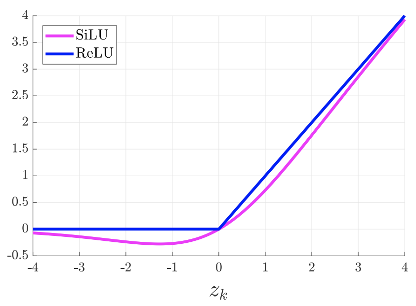
\[b(x) = \text{SiLU}(x) = \frac{x}{1 + e^{-x}}\]

SiLU (Sigmoid Linear Unit) function is an improved version of Sigmoid and ReLU.SiLU has the properties of having no upper and lower bounds, and it is smooth and non-monotonic.SiLU works better than ReLU on deep models. It can be seen as a smooth ReLU activation function.SiLU activation function is also known as the Swish activation function, an adaptive activation function introduced by Google Brain in 2017.

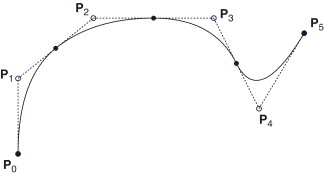
\(\text{spline}(x)\) is parametrized as a linear combination of B-splines such that

\[\text{spline}(x) = \sum_i c_i B_i(x)\]

where every \(c_i\) is trainable. The B-spline function \(\text{spline}(x)\) can be considered a linear combination of control points \(c_i\) and a weighting function \(B_i(x)\). In short, the B-spline curve is the weighted sum of each control point multiplied by its corresponding weight function. The weighting function is predefined and is only related to order D, and it does not change as the control points change.

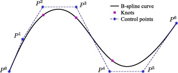
In principle \(w\) is redundant since it can be absorbed into \(b(x)\) and \(\text{spline}(x)\). However \(w\) can better control the overall magnitude of the activation function.

2. Initialization scales:

Each activation function is initialized to have \(\text{spline}(x) \approx 0\).

\(w\) is initialized according to Xavier initialization. Xavier initialization is a very effective method for initializing neural networks, and the method originates from a 2010 paper, Understanding the difficulty of training deep feedforward neural networks.

In the paper, Xavier Glorot offers the insight that the variance of the activation values decreases layer by layer, which results in the gradient in backpropagation and also decreases layer by layer. The solution to the vanishing gradient is to avoid the decay of the variance of the activation values and, ideally, to keep the output values (activation values) of each layer Gaussian distributed. So they initialized the weights \(W\) at each layer with the following commonly used heuristic:

\[W \sim U\left[-\frac{\sqrt{6}}{\sqrt{n_j + n_{j+1}}}, \frac{\sqrt{6}}{\sqrt{n_j + n_{j+1}}}\right]\]

where \(n_j\) is the number of inputs, and \(n_{j+1}\) is the number of outputs.

In addition, each KAN layer has an equal layer width, with L layers and N nodes per layer.

Each spline function is typically of order k = 3, G intervals, and G + 1 grid points.

Thus KANs require a total of \(O(N^2L(G+k))\) or \(O(N^2LG)\) parameters, while MLPs require \(O(N^2L)\) parameters. It may seem that the computational complexity of KANs is greater than that of MLPs, but KANs require much less \(N\) than MLPs, which not only saves parameters but also improves generalization and aids interpretability.

3. Update of spline grids:

In KANs, they update each grid on the fly according to its input activations, to address the issue that splines are defined on bounded regions but activation values can evolve out of the fixed region during training.