Optimal Transport

this is an introduction about Optimal Transport

Intro to Optimal Transport

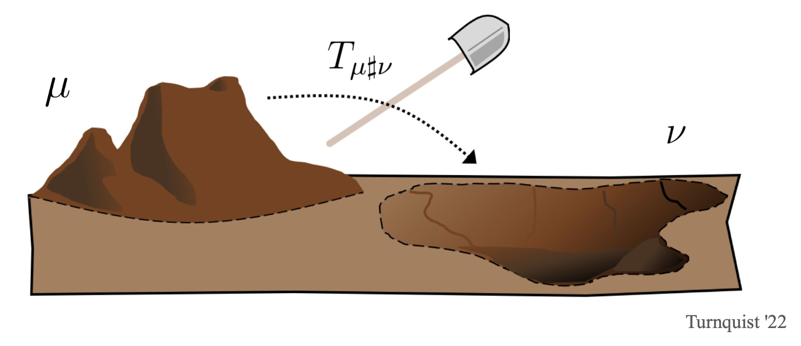
Optimal transport problem can be understood as a problem of two piles of soil, shoveled from soil A to the other and eventually piled up to form soil B. And your mission is to find the most efficient method to shovel the soil.

There are two ways to formulate the optimal transport problem: the Monge and Kantorovich formulations. Historically the Monge formulation comes before Kantorovich. The Kantorovich formulation can be seen as a generalisation of Monge. Both formulations have their advantages and disadvantages. Monge is more useful in applications, whilst Kantorovich is more useful theoretically.

Measure

In mathematics, measure is a generalization and formalization of geometrical measures like length, area, volume, magnitude, mass and probability. In Lebesgue measure, for lower dimensions n = 1, 2, or 3, it coincides with the standard measure of length, area, or volume.

The concept of measures will be used later, and before I introduce probability measures, I need to introduce the histogram. The histogram here is the probability of n sums of 1, representing a probability distribution. We will use interchangeably the terms histogram and probability vector for any element $a \in \Sigma_n $ that belongs to the probability simplex

And we use discrete measure describes a probability measure if, additionally, $a \in \Sigma_n$ and more generally a positive measure if all the elements of vector $a$ are non-negative.

And to avoid degeneracy issues where locations with no mass are accounted for, we will assume when considering discrete measures that all the elements of $a$ are positive.

A convenient feature of OT is that it can deal with measures that are either or both discrete and continuous within the same framework. So we can find a relation between discrete measures and general measures.

The Monge Formulation

In optimal transport, there are two measures $\mu$ and $\nu$. You can imagine they are two piles of soil (but I will call them measure for the rest). And you can also consider the first measure $\mu$ as a pile of sand and the second measure $\nu$ as a hole we wish to fill up. We assume that both measures are probability measures on spaces $X$ and $Y$ respectively. The cost function $c(x,y)$, $c:X \to [0,+\infty]$, measures the cost of transporting one unit of mass from $x \in X$ to $y \in Y$. Now, the problem is to find the most optimal method.

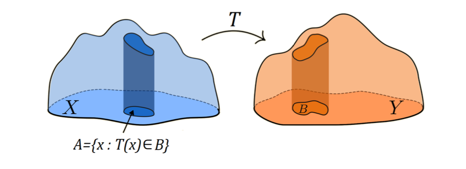
For greter generality we work with the inverse of $T$ itself. The inverse is treated in the general set valued sense, i.e. $x \in T^{-1}(y)$ if $T(x)=y$, if the function $T$ is injective then we can equivalently say that $\nu (T(A)) = \mu (A)$ for all $\mu$-measurable $A$.

Transport map $T$ does not always exist. For example, there are two discrete measures $\mu = \delta_{x_1}$, $\nu = \frac{1}{2} \delta_{y_1} + \frac{1}{2} \delta_{y_2}$, where $y_1 \not= y_2$. Then $\nu({y_1}) = \frac{1}{2}$ but $\mu(T^{-1}(y_1)) \in \{0,1\}$ depending on whether $x \in T^{-1}(y_1)$. Hence no transport maps exist.

The original monge’s optimal transport problem used $L^1$ cost, i.e. $c(x,y) = \mid x - y \mid$. But it is much harder to solve than with $L^2$ cost, i.e. $c(x,y) = \mid x - y \mid^2$.

If the measure is discrete measure, we can also define the Monge’s optimal transport problem between discrete measures.

The Kantorovich Formulation

In the example $\mu = \delta_{x_1}$, $\nu = \frac{1}{2} \delta_{y_1} + \frac{1}{2} \delta_{y_2}$, it causes problem in Monge formulation because mass cannot be split. To allow mass to be split, the Kantorovich formulation appears, which has a natural relaxation. To formalize this, we consider a measure $\pi \in \mathcal{P}(X \times Y)$ and think of $d\pi(x,y)$ as the amount of mass transferred from $x$ to $y$. And we have the constrains:

$\pi(A \times Y) = \mu (A)$, $\pi(X \times B) = \nu (B)$ for all mesaurable sets $A \subseteq X$, $B \subseteq Y$.

And we denote the set of such $\pi$ by $\Pi(\mu,\nu)$ and call $\Pi(\mu,\nu)$ the set of transport plans between $\mu$ and $\nu$. $\Pi(\mu,\nu)$ is never non-empty and $\mu \otimes \nu \in \Pi(\mu,\nu)$. Now we can define Kantorovich’s formulation of optimal transport.

The Kantorovich problem is convex (the constrains are convex and one usually has that the cost functon $c(x,y) = d(x-y)$ where d is convex). And we can also define the Kantorovich problem in discrete measures.

And this is a linear programme. So Kantorovich is considered as the inventor of linear programming.

Wasserstein Distance

When we talk about cost, it is always Eulerian based cost, such as $L^P$, which defines a metric based on “pointwise differences”. However, this cost has some disadvantages. In the optimal transportation process, the probabilities between two points correspond to varying probabilities. Suppose the Euclidean distance is directly used to calculate the loss of transportation (or to measure and evaluate the transportation process). In that case, it will lead to a significant bias in the final evaluation (i.e., directly ignoring the definition of the probability vectors of the original different points).

Optimal transport can be understood as a canonical way to lift a ground distance between points to a distance between historgram or measures. In order to evaluate the goodness of mapped paths for optimal transportation choices, the Wasserstein distance was developed.

To give a clearer idea of what the Wasserstein distance does, suppose the three functions f,g, and h are in the figure below. If you were to represent the distance between f and g and the distance between f and h with L-infinity norm, you would find that the distance between f and g and between f and h are almost the same ($\left \| f-g \right \|_{\infty } \approx \left \| f-h \right \|_{\infty }$). However, under the Wasserstein distance, the distance between f and h is much larger than between f and g ($d_{w_1}(f,q) < d_{w_1} (f,h)$).

The $f, g, h$ functions on $R$:

You can also see the difference between L-infinity norm and Wasserstein distance from the geodesics in the space of functions. If I want to move the function f to the function h, the changes of geodesics in figures below are totally different.

The geodesics under L-infinity norm:

The geodesics under Wasserstein distance:

If we define Wasserstein distance based on the space of probability measures on $X \subset \mathbb{R}^d$ with bounded $p^{th}$ moment, i.e.

If $X$ is bounded then $\mathcal{P}_p(X)=\mathcal{P}(X)$. The Wasserstein distance can be define as

And the wasserstein distance also satisfies the positive definiteness and triangular inequalities of the fugitive space.

Duality

We saw in the previous chapter how Kantorovich’s optimal transport problem resembles a linear programme. It should not therefore be surprising that Kantorovich’s optimal transport problem admits a dual formulation.

In optimization theory, turn original optimizing problem into dual problem can easily make it more easier to solve. Regardless of the difficulty of the original problem, dual problems are convex, and convex problems are a class of problems that are relatively easy to solve. When the original problem is a particularly difficult one, it is relatively easy to solve by reducing it to a dyadic problem

Reminder of Dual Problem

All optimization problems, in theory, can be transformed into standard form:

And then we define Lagrangian function:

\[L(x, \lambda, \mu) = f_0(x) + \sum_{i=1}^{m} \lambda_i f_i(x) + \sum_{j=1}^{p} \mu_j h_j(x)\]

With the Lagrangian function, we introduce the Lagrange dual function:

\[g(\lambda, \mu) = \inf_{x \in \mathcal{D}} L(x, \lambda, \mu)\]

The Lagrange dual function is the Lagrangian function that minimizes with respect to x. And we get the (Lagrangian) dual problem from the standard problem: