Modern Solution of Optimal Transport - Sinkhorn

this is my study note about sinkhorn

Modern Solution of Optimal Transport - Sinkhorn

In 2013, Cuturi proposed a scalable approximation of optimal transport. Since then, OT is increasingly becoming a core tool of machine learning research toolbox.

The computation of other optimal transport formulation involves the resolution of a linear program whose cost can quickly become prohibitive.

But Sinkhorn distance looks at transport problems from a maximum-entropy perspective. It smooths the classic optimal transport problem with an entropic regularization term. And the computation through Sinkhorn’s matrix scaling algorithm is several orders of magnitude faster than that of transport solvers, which is $O(n^2)$.

Sinkhorn Distance

In what follows, $\left \langle \cdot , \cdot \right \rangle$ stands for the Frobenius dot-product. For two probability vectors $\mu$ and $\nu$ in the simplex $\sum_d := \{ x \in \mathbb{R}_+^{d} : x^T \mathbf{1}_d=1 \}$, where $\mathbf{1}_d$ is the d dimensional vector of ones, we write $U(r,c)$ for the transport polytope of $\mu$ and $\nu$, namely the polyhedral set of $d \times d$ matrices,

\[U(\mu,\nu) := \{ P \in \mathbb{R}^{d\times d}_+ | P \mathbf{1}_d = \mu, P^T \mathbf{1}_d = \nu \}\]

And we define the entropy $h$ and Kullback-Leibler divergences of $P,Q\in U(\mu,\nu)$ and a marginals $\mu \in \sum_d$ as

\[h(\mu) = -\sum_{i=1}^{d}\mu_i log \mu_i,\quad h(P) = -\sum_{i,j=1}^{d}p_{ij} log p_{ij}, \quad \mathbf{KL}(P||Q)=\sum_{ij}p_{ij} log\frac{p_{ij}}{q_{ij}}\]

where $p(X=i,Y=j)=p_{ij}$ and the same as $q_ij$.

The following information theoretic inequality (Cover and Thomas, 1991, §2) for joint probabilities

is tight, since the independence table $\mu\nu^T$ has entropy $h(\mu\nu^T) = h(\mu)+h(\nu)$. By the concavity of entropy, we can introduce the convex set

These two definitions are indeed equivalent, since one can easily check that $$\mathbf{KL}(P

\mu\nu^T)= h(\mu)+h(\nu)-h(P)$$, a quantity which is also the mutual information $I(X

Y)$ of two random variables $(X,Y)$ should they follow the joint probability $P$ (Cover and Thomas, 1991, §2).

Why consider an entropic constraint in optimal transport? The first reason is computational. The second reason is built upon the following intuition. As a classic result of linear optimization, the OT problem is always solved on a vertex of $U(\mu,\nu)$. Such a vertex is a sparse $d\times d$ matrix with only up to $2d-1$ non-zero elements (Brualdi, 2006, §8.1.3).

When α is large enough, the Sinkhorn distance coincides with the classic OT distance. When α = 0, the Sinkhorn distance has a closed form and becomes a negative definite kernel if one assumes that M is itself a negative definite distance, or equivalently a Euclidean distance matrix.

And $d_{M,\alpha}(x,y)$ also satisfies the triangle inequality:

\[d_{M,\alpha}(x,z) \le d_{M,\alpha}(x,y)+d_{M,\alpha}(y,z)\]

Computing Regularized Transport with Sinkhorn’s Algorithm

We consider in this section a Lagrange multiplier for the entropy constraint of Sinkhorn distances:

\[For \lambda > 0, d_{M}^{\lambda}(\mu, \nu) := \langle P^{\lambda}, M \rangle, \text{where} \ P^{\lambda} = \underset{P \in U(\mu,\nu)}{\text{argmin}} \langle P, M \rangle - \frac{1}{\lambda}h(P).\]

By duality theory we have that to each $\alpha$ corresponds a $\lambda \in [0,\infty]$ such that $d_{M,\alpha}(\mu, \nu)=d_{M}^{\lambda}(\mu, \nu)$ holds for that pair $(\mu,\nu)$. We call $d_{M}^{\lambda}$ the dual-Sinkhorn divergence and show that it can be computed for a much cheaper cost than the original distance $d_M$.

PyTorch implementation of sinkhorn

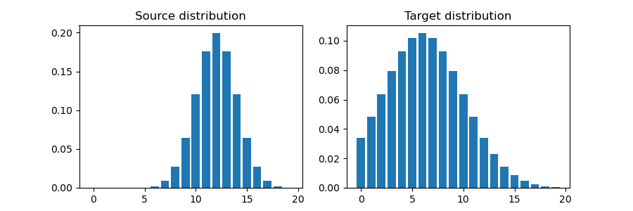
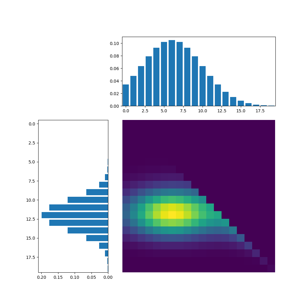
vlkit.optimal_transport.sinkhorn has a PyTorch implementation of sinkhorn that allows us to compute and visualize the optimal transport between two distributions. As an example, two 1d Gaussian distributions are generated as source and target distributions:

import torch
import matplotlib
import matplotlib.pyplot as plt
from matplotlib import gridspec
from vlkit.optimal_transport import sinkhorn

# generate two gaussians as the source and target
def gaussian(mean=0, std=10, n=100):
    d = (-(torch.arange(n) - mean)**2 / (2 * std**2)).exp()
    d /= d.sum()
    return d

n = 20
d1 = gaussian(mean=12, std=2, n=n)
d2 = gaussian(mean=6, std=4, n=n)

dist = (torch.arange(n).view(1, n) - torch.arange(n).view(n, 1)).abs().float()
dist /= dist.max()

# visualize distr
fig, axes = plt.subplots(1, 2, figsize=(9, 3))
axes[0].bar(torch.arange(n), d1)
axes[0].set_title('Source distribution')
axes[1].bar(torch.arange(n), d2)
axes[1].set_title('Target distribution')
plt.tight_layout()

T, u, v = sinkhorn(r=d1.unsqueeze(dim=0), c=d2.unsqueeze(dim=0), reg=1e-2, M=dist.unsqueeze(dim=0))
plt.figure(figsize=(10, 10))
gs = gridspec.GridSpec(3, 3)

ax1 = plt.subplot(gs[0, 1:3])
plt.bar(torch.arange(n), d2, label='Target distribution')

ax2 = plt.subplot(gs[1:, 0])
ax2.barh(torch.arange(n), d1, label='Source distribution')

plt.gca().invert_xaxis()
plt.gca().invert_yaxis()
plt.subplot(gs[1:3, 1:3], sharex=ax1, sharey=ax2)
plt.imshow(T.squeeze(dim=0))
plt.axis('off')
plt.tight_layout()